Colored cells in Microsoft Excel can help you organize data, track changes, and make it easier to read. For example, in a customer spreadsheet, you might use a green background to track which customers have made a sale. But how do you count these colored cells?
Method 1: Count Colored Cells With Find and Select

Excel includes a Find and Select feature that lets you count cells of different colors. Here’s how to use it:
- Select the Home tab then press the magnifying glass icon.
- In the drop-down menu, select Find…
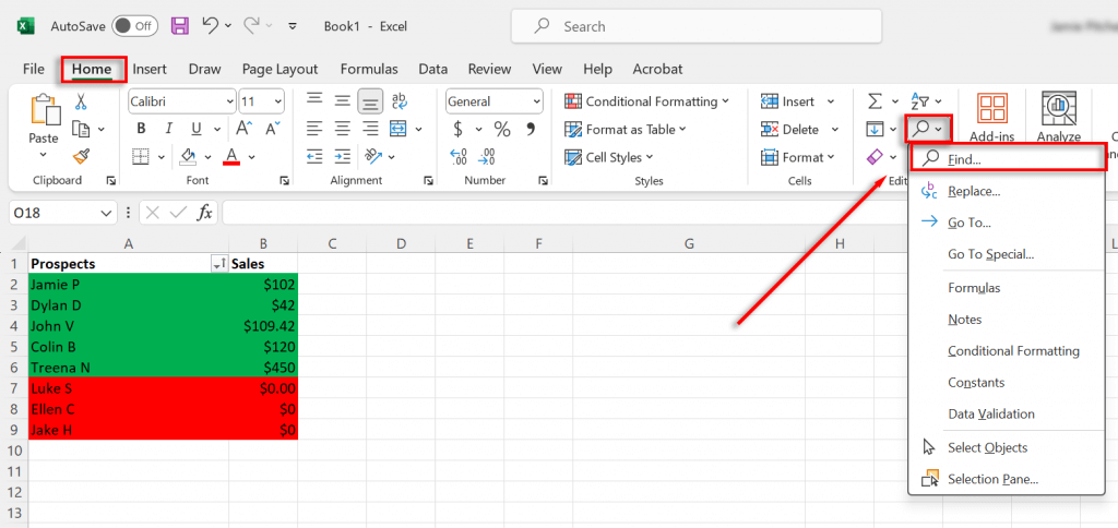
- Select the Format… drop-down menu and choose Choose Format From Cell…
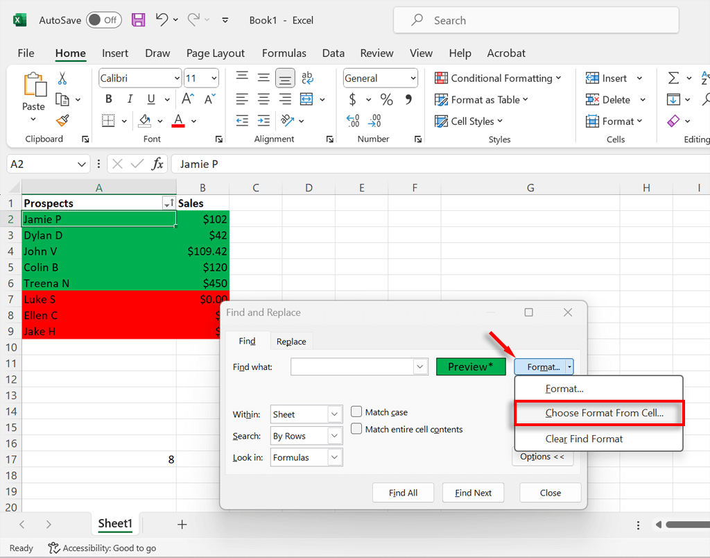
- Use the cursor to select a cell in the color you want to count.
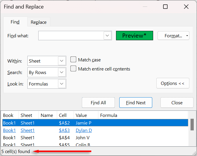
- Select Find All . Excel will then display a list of all the cells in your workbook that are of the same color. Below the list, to the bottom-left, there will be a final count of these colored cells.
Method 2: Count Colored Cells Using the Subtotal Function
The subtotal function lets you count the number of formatted cells according to data filters. Here’s how to use the filter function to count colored cells:
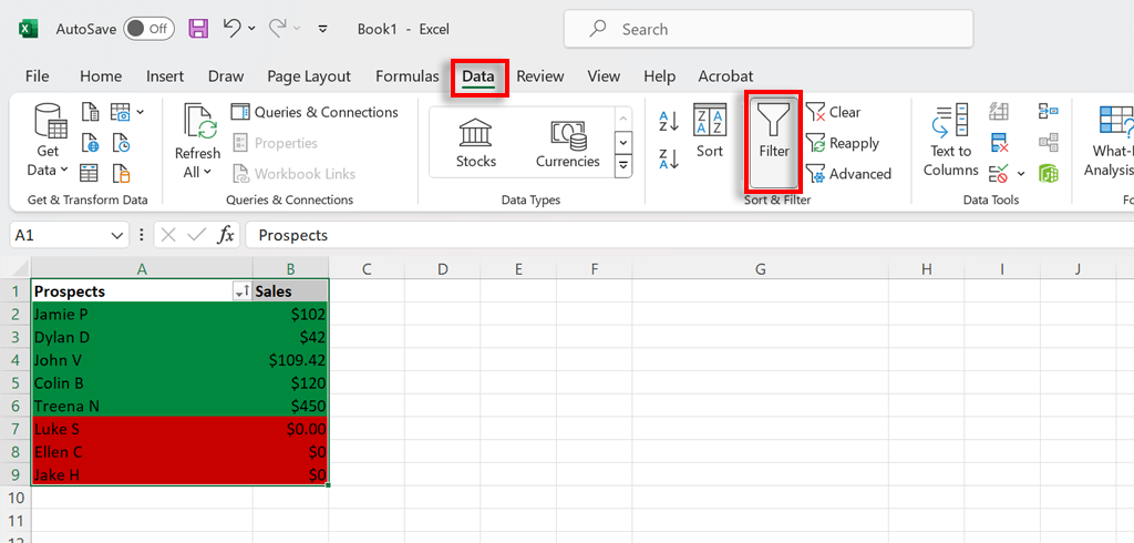
- Select all of your data by pressing Ctrl + A .
- Press the Data tab , then select Filter . This will add gray drop-down menus to each of your columns that contain data.
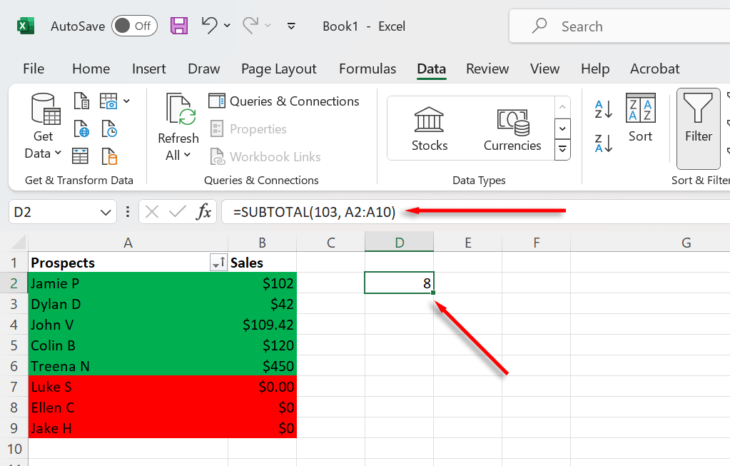
- Choose an empty cell and enter the subtotal formula, which is =SUBTOTAL(Function_num, Ref1) .
- Replace Function_num, with “102.” This tells Excel to count cells with numbers, not including hidden cells. If your cells are words, as in our example, use “103” – this counts cells with any value within them. For Ref1, you need to select the range of data you want Excel to count. So in this case, it would be:
=SUBTOTAL(103, A2:A10)
<img loading=“lazy” src=“https://helpdeskgeek.com/wp-content/pictures/2024/04/how-to-count-colored-cells-in-excel-sheets-6-compressed.png" onerror=“this.onerror=null;this.src=‘https://blogger.googleusercontent.com/img/a/AVvXsEhe7F7TRXHtjiKvHb5vS7DmnxvpHiDyoYyYvm1nHB3Qp2_w3BnM6A2eq4v7FYxCC9bfZt3a9vIMtAYEKUiaDQbHMg-ViyGmRIj39MLp0bGFfgfYw1Dc9q_H-T0wiTm3l0Uq42dETrN9eC8aGJ9_IORZsxST1AcLR7np1koOfcc7tnHa4S8Mwz_xD9d0=s16000';" alt=“Type “=SUBTOTAL(103, A2:A10)”, replacing each field with the relevant data for your sheet - 6”>
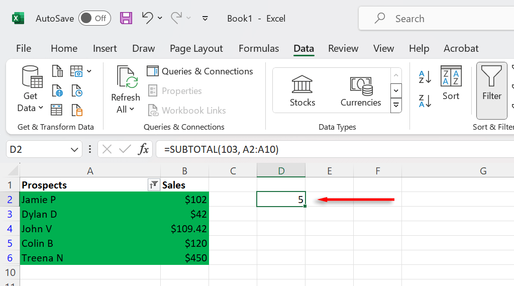
- The subtotal equation should calculate the total number of cells. For this to work, you’ll need to use cells with numbers in them.
- Press the Filter drop-down menu and choose Filter by Color . Choose the color you want to filter by.
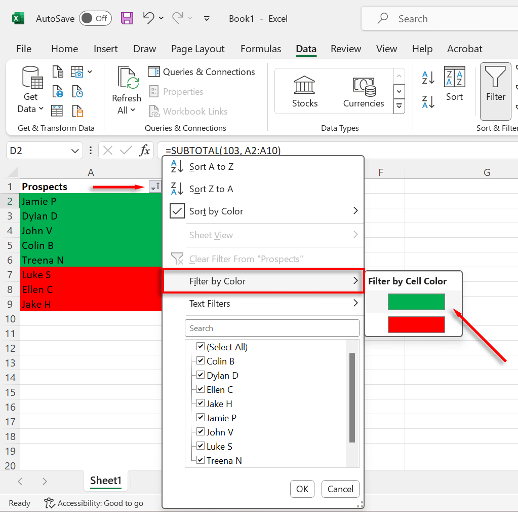
- The subtotal will now display the total number of cells in that color.
Note: If you’re struggling to get the formulas above to work, try learning about function syntax in Microsoft Excel. Once you understand how the syntax works, you’ll be able to troubleshoot any problems you’re having easily.
Counting Colored Cells Made Easy
Hopefully, you can now count your colored cells in Excel easily. While there are other ways to count cells, including complicated formulas and custom VBA functions , they are generally not worth the effort.
- How to Find Circular References in Microsoft Excel
- Name Box in Excel: All You Need to Know
- How to Remove Unwanted Spaces from Excel Spreadsheets
- How to Unhide the First Column or Row in Excel Worksheets
- How to Use the Square Root (SQRT) Function in Excel
Jake Harfield is an Australian freelance writer whose passion is finding out how different technologies work. He has written for several online publications, focusing on explaining what he has learned to help others with their tech problems. He’s an avid hiker and birder, and in his spare time you’ll find him in the Aussie bush listening to the birdsong. Read Jake’s Full Bio
